How to calibrate coalescent trees to geological time
There has been much interest recently in using the multi-species coalescent to estimate species phylogenies from molecular data. The advantage of the method is that incomplete lineage sorting (the discrepancy between gene trees and the species tree), and ancestral polymorphism are accounted for during phylogenetic inference. Bayesian implementations of the method are computationally expensive, and are best suited for inference among closely related species (or populations).
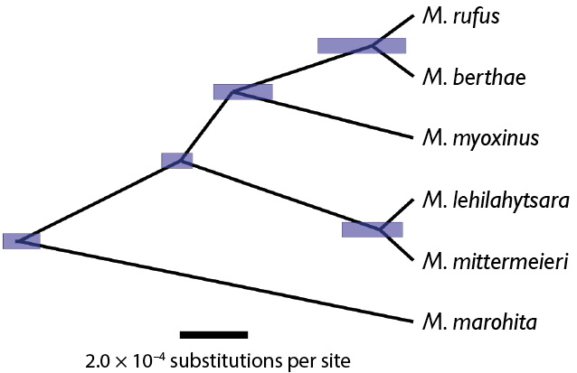
The figure below shows an example of a phylogeny of mouse lemurs (Microcebus spp.) estimated from RADseq (restriction site associated DNA sequencing) data using the program BPP (Yang, 2015), which implements the multi-species coalescent. Each node in the tree represents a speciation event, with the node ages given as numbers of substitutions per site. The blue bars represent the 95% credibility interval of the node age. For example, the molecular distance from the last common ancestor of M. rufus and M. berthae to the present is 1.29 × 10⁻⁴ substitutions per site. If we knew the molecular substitution rate per year for mouse lemurs, we could calibrate the tree to geological time, that is, we could convert the node ages from units of substitution per site to units of real time. I’ll explain how to do so in this post.
A simple method
The mouse lemur genome is roughly 2.8 Gbp long, with perhaps the majority of the genome evolving neutrally. The RADseq data used to build the phylogeny above represents a random sample of the genome, and thus we may assume that most RAD-fragments are evolving neutrally. Estimates of the de novo mutation rate in the human genome are around 1.2 × 10⁻⁸ substitutions per site per generation (see Scally and Durbin, 2012, for a review). Given that mouse lemurs are also primates, we could use the human mutation rate as a proxy for the mouse lemur rate. Assuming a generation time of 4 years for mouse lemurs would roughly give us 1.2 × 10⁻⁸ / 4 = 0.3 × 10⁻⁸ substitutions per site per year for the lemur rate. Let τ be the age of a node in the phylogeny in units of substitutions per site. Then it follows that τ = rt, where r is the mutation rate per year, and t the age in years. For the M. rufus and M. berthae divergence we have that τ = 1.29 × 10⁻⁴, and thus t = τ/r = 1.29 × 10⁻⁴ / 0.3 × 10–8 = 43,000 years. We could repeat the procedure to the other nodes in the tree to obtain all the ages of divergence. This is perhaps the simplest procedure to calibrate a coalescent tree to geological time.
The procedure outlined above has at least two serious limitations however. The first is that we used point estimates for τ and the mutation rate, r, and we have thus ignored the uncertainties associated with these estimates. The second is that the human mutation rate is probably not a good proxy for the mouse lemur rate. We now look at a more sophisticated way to calibrate the tree that overcomes these issues.
A full Bayesian approach
The following discussion assumes you have a basic grasp of Bayesian statistics, are familiar with BPP (or other similar Bayesian coalescent inference software), and with the R environment for statistical computing.
The program BPP uses an MCMC Bayesian approach to estimate the model parameters (i.e. the species phylogeny, the ancestral nucleotide diversities, θ = 4Nu, and the τ’s) from a molecular sequence alignment. Once an MCMC BPP analysis has finished, one obtains a sample of the posterior distribution of the parameters of interest. The sample size is specified by the user when running the software. For example, for the tree above I analysed 80,662 RAD-fragments and took 20,000 samples from the MCMC (see Yoder et al., 2016, for details). In fact, because the analysis is so computationally intensive, I actually ran 8 parallel MCMC analysis, each with 20,000 samples. Here I discuss the results from only one of those analysis, but the results presented in the main paper by Yoder et al. were calculated using all 8 × 20,000 = 160,000 samples.
To obtain a full Bayesian estimate of the divergence times of the mouse lemurs we must first construct priors on the per-generation mutation rate, u; and the generation time in years, g. One can then obtain samples from these priors, which can then be combined with the samples of τ’s from BPP to obtain the desired divergence times (Angelis and dos Reis, 2015). Let τi be the i-th sample of a node age from the MCMC, and ui, and gi the i-th sample obtained from the priors. Then, the i-th sample of the mutation rate per year is given by ri = ui / gi. Finally, the i-th sample of the divergence time in years is ti = τi / ri. Thus, one simply repeats the procedure for as many times as the MCMC sample size to obtain the full posterior distribution of t. The whole procedure is then repeated for the other nodes in the phylogeny. Below I exemplify the procedure using the mouse lemur phylogeny.
A prior on the mouse lemur generation time: Considerations of the reproductive biology and lifespan in wild and captive populations of mouse lemurs give an estimate of 3 to 4.5 years for the generation time in this species (Yoder et al. 2016). Thus we can construct a gamma prior for g with mean 3.75 years (the mid-point of 3–4.5) and standard deviation 0.375 years (so that 3.75 ± 2 × 0.375 equates to 3–4.5 years). Recall that the gamma distribution with parameters α and β has mean α/β and variance α/β2. Thus, the prior for g is
f (g) = Gamma (g | α = 100, β = 26.67). (1)
A prior on the mouse lemur per-generation mutation rate: Estimates of the mutation rate in the lab mouse are about 0.54 × 10⁻⁸ substitutions per site per generation (Uchimura et al. 2015), while, as mentioned above, they are about 1.2 × 10⁻⁸ substitutions per site per generation in human. It is unclear whether the per-generation mutation rate in the mouse lemurs should be similar to the lab mouse (which has a similar body size and lifespan), or to the human (a fellow Primate), thus, we construct a conservative gamma prior on u between 0.5–1.2 (× 10–8) substitutions per site per generation. Using the same procedure as above, we get a mean of 0.87 (× 10–8) substitutions per site per generation, and a standard deviation of 0.165 (× 10–8) substitutions per site per generation. The prior on u is then
f (u) = Gamma (u | α = 27.80, β = 31.96). (2)
Converting the τ’s into geological times of divergence: The table below summarises the procedure. The first column (i) indicates the sample number. The second column (τrb) is the MCMC posterior sample obtained with BPP of the age of the M. rufus and M. berthae divergence. The third column (u), is the sample of the per-generation mutation rate from the gamma prior of Eq. (1). I generated the sample of u using R, that is, by running the R command rgamma(2e4, 27.80, 31.96). The fourth column (g), is the sample of the generation time from the gamma prior of Eq. (2), also obtained with R. The fifth column (r) is the prior sample of the per-year mutation rate, obtained by combining the priors on u and g. Finally, the last column (trb) is the resulting sample of the posterior distribution of the geological time of divergence of M. rufus and M. berthae, obtained by combining the prior on r with BPP’s posterior of τrb. One can summarise the posterior sample of trb in the usual way, to obtain the posterior mean, variance, and 95% credibility interval (CI). The posterior mean is 57,545 years before present with 95% CI: 142,193–10,207 years. The table below can be uploaded into a program such as Tracer, to analyse the traces of r and trb, calculate the ESS, etc.
| i | τrb (× 10–4) | u (× 10–8) | g | r (= u/g × 10–8) | trb (= τ/r) |
|---|---|---|---|---|---|
| 1 | 1.632 | 0.742 | 4.109 | 0.181 | 90,372 |
| 2 | 1.531 | 0.903 | 4.033 | 0.224 | 68,378 |
| 3 | 1.566 | 1.124 | 2.956 | 0.380 | 41,165 |
| . . . | . . . | . . . | . . . | . . . | . . . |
| 20,000 | 1.599 | 0.758 | 3.673 | 0.206 | 77,473 |
The advantage of the procedure just outlined is that one obtains the full, correct posterior distribution of the divergence times integrating all the uncertainties involved. Note that this procedure allows the use of arbitrary prior distributions for u and g (as long as one can obtain samples for them) without having to make any complex analytical calculations. The procedure can be easily extended to calculate the ancestral effective population sizes, N, from BPP’s posterior sample of the nucleotide diversities (θ = 4Nu). The reader should be able to work out how to do this easily. The method can also be trivially extended to deal with the output of other programs and methods (such as, for example, the pairwise sequentially Markovian coalescent or PSMC).
You can read more about our mouse lemur research, and see how estimating their times of divergence let us get a glimpse of Madagascar’s forests past, at The Washington Post and National Geographic.
The files and code needed to reproduce this tutorial are available from github.com/mariodosreis/mousies.
References
Angelis K, and dos Reis M. (2015) The impact of ancestral population size and incomplete lineage sorting on Bayesian estimation of species divergence times. Current Zoology, 61: 874–885.
Scally A, and Durbin R. (2012) Revising the human mutation rate: implications for understanding human evolution. Nature Reviews Genetics, 13: 745–753.
Uchimura A, et al. (2015) Germline mutation rates and the long-term phenotypic effects of mutation accumulation in wild-type laboratory mice and mutator mice. Genome Research, 25: 1125–1134.
Yang Z. (2015) The BPP program for species tree estimation and species delimitation. Current Zoology, 61: 854–865.
Yoder AD, et al. (2016) Geogenetic patterns in mouse lemurs (genus Microcebus) reveal the ghosts of Madagascar’s forests past. Proceedings of the National Academy of Sciences, 113: 8049–8056.