Estimating the marginal likelihood of a relaxed-clock model with MCMCTree
MCMCTree now implements MCMC sampling from power-posterior distributions. This allows estimation of the marginal likelihood of a model for Bayesian model selection –that is, by calculation of Bayes factors or posterior model probabilities. In MCMCTree, this allows selection of the relaxed-clock model for inference of species divergence times using molecular data (dos Reis et al. 2017).
To calculate the marginal likelihood of a model, one must take samples from the so-called power-posterior, which is proportional to the prior times the likelihood to the power of b, with 0 ≦ b ≦ 1. When b = 0, the power posterior reduces to the prior, and when b = 1, it reduces to the normal posterior distribution. Thus, by selecting n values of b between 0 and 1, one can sample likelihood values from the power posterior in a path from the prior to the posterior. The sampled likelihoods are then used to estimate the marginal likelihood either by thermodynamic integration (a.k.a. path sampling) or by the stepping stones method. Applications of both methods are extensive in the phylogenetics literature (Lartillot and Philippe 2006, Lepage et al. 2007, Xie et al. 2011). A review of Bayesian model selection is given in Yang (2014).
Tutorial
This tutorial introduces the user to marginal likelihood calculation in MCMCTree to select for a relaxed-clock model. MCMCTree (v4.9f at the time of writing) implements three clock models: the geometric Brownian motion (GBM) model, the independent log-normal (ILN) model, and the strict clock (CLK) model (Rannala and Yang, 2007). I have written an R package mcmc3r (available in GitHub) which helps the user in selecting appropriate b values, preparing the corresponding MCMCTree control files, and in parsing MCMCTree’s output to calculate the marginal likelihood. This tutorial assumes the user has basic knowledge of MCMCTree and Bayesian divergence time estimation, and a basic understanding of Bayes factors and marginal likelihood theory. It also assumes you have basic knowledge of R, and have the devtools and coda R packages installed. The tutorial has been tested on MacOS, but it should work in other systems (e.g. Linux or Windows), although some tweaking may be necessary.
You can download MCMCTree, which is part of the PAML phylogenetic analysis package, from Ziheng Yang’s website. You should place the mcmctree excecutable in your system’s search path as explained in the website.
Update – 2026: Ziheng’s personal website is no longer active. To download MCMCtree please use the official PAML GitHub Repository. In the GitHub page, please read the section on “Downloading an installing PAML” including the parts on exporting the path variable for your particular system (i.e., Windows, Linux, Mac).
The mcmc3r package can be installed in R by typing
devtools::install_github ("dosreislab/mcmc3r")
The general procedure to calculate Bayes factors with MCMCTree is as follows:
-
Select the sequence alignment and phylogenetic tree to be analysed.
-
Prepare a template
mcmctree.ctlfile with values for the appropriate relaxed-clock model, priors, alignment and tree files. -
Use
mcmc3rto select n appropriate b values according to the marginal likelihood calculation method of choice (stepping stones or thermodynamic integration) and prepare n directories with correspondingmcmctree.ctlfiles. -
Run MCMCTree n times, to sample from the n power posteriors.
-
Use
mcmc3rto parse MCMCTree’s output and calculate the marginal likelihood for the chosen relaxed-clock model. -
Repeat 2-5 for other clock models as necessary.
-
Calculate Bayes factors and posterior model probabilities.
1. Alignment and tree
The data to be analysed are the 15,899 nucleotides alignment of the mitochondrial genomes of four ape species (human, Neanderthal, chimp and gorilla). The alignment ape4s.phy and tree ape4s.phy, as well as the mcmcmtree.ctl template, are available within the misc/ directory in the R package. Make a directory called ape4s/ and copy the alignment, and tree files into it.
Using a text editor you can look into the alignment file. The alignment, which is compressed into site patterns, is shown below:
        4         86  P

Ggor                            AAAAAAAAAA AAAAAAAAAA AAAAAAACCC CCCCCCCCCC CCCCCCCCCC CCCGGGGGGG GGGGGGGGTT TTTTTTTTTT TTTTTT
Hnea                            AAAAAAACCC CCCCGGGGGG TTTTTTTAAA AAAACCCCCC CCGGGGTTTT TTTAAAACCC CGGGGGTTAA AACCCCCCGG GTTTTT
Hsap                            AAAAGGTACC CTTTAAGGGG AACTTTTAAA AGGTACCCCG TTAGGGCCCT TTTAAGGCCC CAAGGGTTAA AACCCGTTGG GCCTTT
Ptro                            ACGTAGAAAC TACTAGACGT ATTACGTACG TACTCACGTA CTAACGACTA CGTAGAGACG TAGACGATAC GTACTCCTAG TCTACT


4423   10  136   13   27    1    1    1   12   34    8    1    2    1   28
   5  131    1   59    1    1    1    1    9    5    1   12   28   13    2
   5    1    1    1    1   11 4028    3  261    1   18    5    1    1    1
   4    1   16   11    2  233    1  220  166   28    3    5    3    1    1
   4   10    3   51    2 1793    1    3   32    2    5    3    1  368  169
   1    7    6    2    2    1    7   14    6  120 3284
The first line gives the number of species (4), the number of site patterns (86) and a ‘P’ indicating it is a compressed alignment. The next block shows the four species and corresponding nucleotide sequences. The last block shows the number of times each site pattern is seen in the alignment. The sum of these numbers is 15,899, the alignment length. See PAML’s manual for alignment formats.
The tree file is:
4 1
(((Hsap, Hnea), Ptro), Ggor)'B(0.999,1.001)';
The first line indicates the number of species (4), and the number of trees in the file (1), then the tree in Newick format is given. Because our interest is to select the relaxed-clock model and not to estimate absolute divergence times, we will fix the age of the root to one. In MCMCTree this is done by labelling the root with B(0.999,1.001), which tells MCMCTree that the age of the root is constrained to be between 0.999 and 1.001. See MCMCTree’s manual for calibration formats.
2. Preparing the MCMCTree template
The first clock model that we will test is the strict clock (CLK). Create a directory ape4s/clk/ and copy the misc/mcmctree.ctl file into it. The MCMCTree template file is shown below:
seed = -1
seqfile = ../../ape4s.phy
treefile = ../../ape4s.tree
outfile = out

ndata = 1      * number of partitions
usedata = 1    * 0: no data; 1:seq like; 2:use in.BV; 3: out.BV
clock = 1      * 1: global clock; 2: independent rates; 3: correlated rates

model = 4    * 0:JC69, 1:K80, 2:F81, 3:F84, 4:HKY85
alpha = .5   * alpha for gamma rates at sites
ncatG = 5    * No. categories in discrete gamma

BDparas = 1 1 0      * birth, death, sampling
kappa_gamma = 2 .2   * gamma prior for kappa
alpha_gamma = 2 4    * gamma prior for alpha

rgene_gamma = 2 20   * gamma prior for mean rates for genes
sigma2_gamma = 1 10  * gamma prior for sigma^2 (for clock=2 or 3)

print = 1
burnin = 4000
sampfreq = 6
nsample = 20000
For a detailed explanation of all the options in the file please refer to MCMCTree’s manual. Note that the clock model is set to clock = 1 which is the model we will test first.
3. Selecting the b values with mcmc3r
Open a terminal window, change into the clk/ directory and start R. Make sure that clk/ is R’s current working directory. We will select 8 b points to estimate the marginal likelihood of CLK using the stepping stones method. In R, type:
b = mcmc3r::make.beta(n=8, a=5, method="step-stones")
The 8 b values range from 0 to 0.5129. Constant a controls the distribution of b between 0 and 1. Large a values produce b values clustered close to zero, which is desirable for large sequence alignments.
We now construct 8 directories each containing a modification of the mcmctree.ctl template. In R type:
mcmc3r::make.bfctlf(b, ctlf="mcmctree.ctl", betaf="beta.txt")
ctlf specifies the template control file, and betaf is the name of a file that will contain the selected b values. Open a new terminal window and look at the contents of clk/. You will see the 8 new directories created together with the beta.txt file. Each directory contains the mcmctree.ctl file with an additional line. For example, the last line of 8/mcmctree.ctl is
BayesFactorBeta = 0.512908935546875
which tells MCMCTree to sample from the power posterior with b = 0.5129 … . Note that MCMCTree currently cannot sample log-likelihoods using b = 0, and so b = 10–300 (a tiny number) is used instead (i.e. look into 1/mcmctree.ctl).
4. Run MCMCTree
Now run MCMCTree within each one of the 8 directories created in the previous step. The following Bash command does the trick in the Mac:
for d in `seq 1 1 8`; do cd $d; mcmctree >/dev/null & cd ..; done
It takes about 40s for the 8 MCMCTree runs to finish on a 2.8 GHz Intel Core i7 machine with four processors. For analysis of larger alignments, and in particular with richer taxon sampling, computation time will be substantially longer. In such cases it may be desirable to prepare a customised script and submit the MCMCTree jobs to a high-throughput computer cluster.
5. Parse MCMCTree’s output with mcmc3r
Go back to the terminal where you are running R. Type:
clk <- mcmc3r::stepping.stones()
clk$logml; clk$se
# $logml
# [1] -32185.72
# $se
# [1] 0.03516095
The stepping.stones() function will read the b values in beta.txt and will read the log-likelihood values sampled by MCMCTree within each directory. It will then compute the log-marginal likelihood and its standard error.
The log-marginal likelihood estimate for CLK is –32,185.72 with a standard error (S.E.) of 0.035. Note that your values may be slightly different due to the stochastic nature of the MCMC algorithm. The S.E. can be used to construct a 95% confidence interval for the estimate: –32,185.72 ± 2×0.035. Ideally, you want the S.E. to be much smaller than the log-marginal likelihood difference between the models being tested. You may reduce the S.E. by increasing nsample or samplefreq in the mcmctree.ctl template file. Note that to reduce the S.E. by half, you need to increase nsample four times.
6. Repeat for the ILN and GBM models
Go back to ape4s/ and create directories called iln/ and gbm/. Copy the mcmctree.ctl template into each directory, and modify the templates appropriately. For the ILN model, you must set clock = 2 (independent rates) in the template, and for the GBM model, it must be set to clock = 3 (correlated rates). Repeat steps 3 to 5 for both models. In R:
# This assumes you are currently in clk/
setwd("../iln")
# prepare templates for ILN:
mcmc3r::make.bfctlf(b, ctlf="mcmctree.ctl", betaf="beta.txt")
setwd("../gbm")
# prepare templates for GBM:
mcmc3r::make.bfctlf(b, ctlf="mcmctree.ctl", betaf="beta.txt")
In the terminal:
# This assumes you are currently in clk/
cd ../iln; for d in `seq 1 1 8`; do cd $d; mcmctree >/dev/null & cd ..; done
cd ../gbm; for d in `seq 1 1 8`; do cd $d; mcmctree >/dev/null & cd ..; done
Once the MCMCTree jobs have finished, return to your R session:
setwd("../iln"); iln <- mcmc3r::stepping.stones()
setwd("../gbm"); gbm <- mcmc3r::stepping.stones()
The estimated log-marginal likelihoods and S.E.’s for the three models are:
| CLK: | –32,185.72 | ± 0.035 |
| ILN: | –32,186.69 | ± 0.045 |
| GBM: | –32,186.20 | ± 0.060 |
7. Calculate Bayes factors and posterior model probabilities
Now we can calculate the Bayes factors and posterior model probabilities easily with R:
# log-marginal likelihoods for CLK, ILN and GBM:
mlnl <- c(clk$logml, iln$logml, gbm$logml)
# mlnl: -32185.72, -32186.69, -32186.20

# Bayes factors
( BF <- exp(mlnl - max(mlnl)) )
# [1] 1.0000000 0.3790830 0.6187834

# Posterior model probabilities
( Pr <- BF / sum(BF) )
# [1] 0.5005340 0.1897439 0.3097221

# or alternatively:
mcmc3r::bayes.factors(clk, iln, gbm)
The posterior probabilities are calculated assuming equal prior model probabilities. The CLK model has the highest log-marginal likelihood, and thus the highest posterior probability (Pr = 0.50), followed by GBM (Pr = 0.31), with ILN being the worst performing model (Pr = 0.19). This result should not be surprising. Human, Neanderthal, chimp and gorilla are all very closely related, and the strict clock is usually not rejected in comparisons of such closely related species. Indeed, a likelihood-ratio test fails to reject the strict clock in this data (see Box 2 in dos Reis et al. 2016 where the data are analysed).
Update – Feb 2020: Function bayes.factors now performs parametric bootstrap of posterior probabilities, so you should see an element called $pr.ci with the confidence intervals for the posterior probabilities.
Update - Dec 2020: For large datasets, MCMC sampling of power posteriors can be quite time consuming. In such cases, a good strategy may be to run shorter MCMC chains and more frequent sampling, for example using nsample = 10000 and samplefreq = 2 in the control file. To compensate for the shorter chains, one may then use many more beta points (for example 32 or 64). However, in such cases, the delta approximation used to calculate the S.E. (see Xie et al. 2011) may not work well due to the smaller sample size. Instead, we can use the stationary block bootstrap method of Politis and Romano (1994) to calculate the S.E. New functions are now provided in the package to do this. In R:
r <- 100 # we will use 100 bootstrap replicates
setwd("../clk")
mcmc3r::block.boot(r) # generate bootstrap replicates
# (for each beta value, replicates are stored in files lnL1.txt to lnL100.txt,
# with lnL0.txt containing the original log-likelihood values)
clk.boot <- mcmc3r::stepping.stones.boot(r) # calculate logml on the replicates

# repeat for the iln and gbm models
setwd("../iln")
mcmc3r::block.boot(r); iln.boot <- mcmc3r::stepping.stones.boot(r)
setwd("../gbm")
mcmc3r::block.boot(r); gbm.boot <- mcmc3r::stepping.stones.boot(r)

# You can now look at the S.E.'s calculated using the bootstrap samples
clk.boot$se; iln.boot$se; gbm.boot$se

# calculate bayes factors and posterior model probabilities
mcmc3r::bayes.factors(clk.boot, iln.boot, gbm.boot)
Function block.boot uses the MCMC sample of power likelihoods to generate new pseudo-MCMC samples of likelihoods. This is done by extracting, with replacement, blocks of consecutive likelihood values within each power posterior MCMC. The block sizes are random and have a geometrical distribution. The sampled blocks are then stitched together to form the pseudo-MCMC sample. This is necessary because the MCMC is a stationary autocorrelated time series and the standard bootstrap method cannot be used. Politis and Romano (1994) show the method works well to approximate the distribution of statistics of stationary time series. The stepping.stones.boot function goes through the r=100 bootstrap replicates and calculates a marginal likelihood on each replicate. These in turn are used to obtain the S.E. and a 95% C.I. for the original log-marginal likelihood estimate.
In our example here, the S.E.’s from the block boot method are quite close to those from the delta method, and the 95% CI’s on the posterior model probabilities, Pr(M|D), are virtually identical:
| M | –log L | S.E. (delta) | S.E. (boot) | Pr(M|D) | 95% CI (delta) | 95% CI (boot) |
|---|---|---|---|---|---|---|
| CLK | 32,185.72 | ± 0.035 | ± 0.034 | 0.500 | (0.47, 0.53) | (0.47, 0.53) |
| ILN | 32,186.69 | ± 0.045 | ± 0.043 | 0.190 | (0.17, 0.21) | (0.17, 0.21) |
| GBM | 32,186.20 | ± 0.060 | ± 0.068 | 0.310 | (0.28, 0.34) | (0.28, 0.34) |
For short MCMC chains the delta method’s S.E. estimates will deteriorate rapidly, but those from the boot method will be more reliable.
Thermodynamic integration with Gaussian quadrature
You can repeat steps 3 to 7 using the thermodynamic integration method. Make sure you create a new set of clk/, iln/ and gbm/ directories to run the analyses. In step 3, generate the b values and directories using R with:
b = mcmc3r::make.beta(n=32, method="gauss-quad")
mcmc3r::make.bfctlf(b, ctlf="mcmctree.ctl", betaf="beta.txt")
This will select b values using the n-Gauss-Legendre quadrature rule (see Rannala and Yang, 2017, for details) and prepare the necessary mcmctree.ctl files. Note that we are using n = 32 points. Then continue with step 4 to run MCMCTree. In step 5, you again use R to parse MCMCTree’s output for the CLK model, but this time you use a different function:
clk <- mcmc3r::gauss.quad()
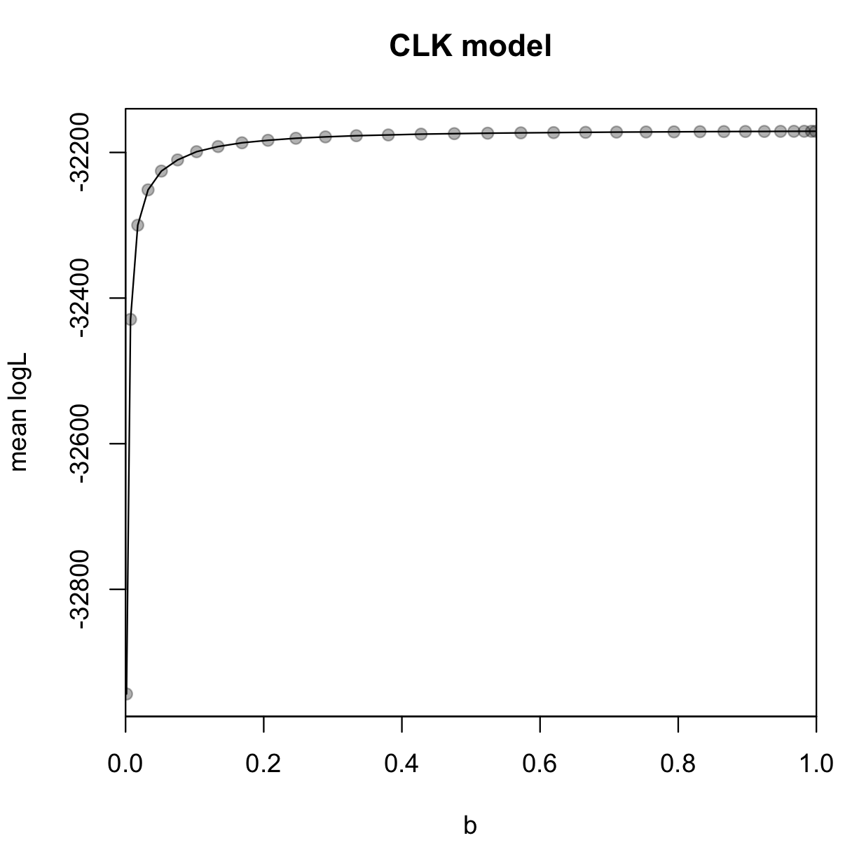
In the thermodynamic integration method, the log-marginal likelihood is the integral of the path formed by the mean log-likelihoods sampled as a function of the b value used (that is, the area above the path, between the path and zero). You can plot this easily in R:
plot(clk$b, clk$mean.logl, pch=19, col=rgb(0,0,0,alpha=0.3), xaxs="i",
     xlim=c(0,1), xlab="b", ylab="mean logL", main="CLK model")
lines(clk$b, clk$mean.logl)
You can now repeat step 6 to calculate the marginal likelihoods for the ILN and GBM models, and then repeat step 7 to obtain the posterior model probabilites. The log-marginal likelihood estimates and S.E.’s are:
| CLK: | -32,185.66 | ± 0.023 |
| ILN: | -32,186.61 | ± 0.036 |
| GBM: | -32,188.17 | ± 0.055 |
The log-marginal likelihood estimates here are very close to those obtained under the stepping stones method. However, note we used n = 32 points to converge to the same result as with stepping stones. Thus, the stepping stones method appears more efficient. Note the S.E. only gives you an idea of the precision, not the accuracy, of the estimate. It is possible to obtain very precise estimates of the marginal likelihood (the S.E. is very small) that are biased (i.e. the estimate is far from the true value). This is due to the discretisation bias in the calculation of the ‘thermodynamic’ integral (see Lartillot and Philippe 2006, and Xie et al. 2011). This will occur especially if n is small. Try n = 1 (which performs very poorly).
Other applications of Bayes factors in MCMCTree
The strategy used here to select for a relaxed-clock model can also be used to select for the tree topology or the substitution model.
Say you have 3 competing tree topologies, and you want to calculate the posterior probability of each. You can prepare 3 Newick files with the different topologies, and create 3 directories, into which you will run the three separate marginal likelihood calculations. In this case you would prepare 3 mcmctree.ctl templates, with the same parameters for all analyses, except for the treefile variable, which you would edit to point to the appropriate tree topology. The rest of the procedure is then exactly the same as when selecting for the relaxed-clock model.
A similar approach can be used to select for a substitution model. Say you want to compare HKY85 vs. HKY85+Gamma. In this case you would have two mcmctree.ctl templates, differing only in the alpha variable in the template (alpha=0 for no Gamma model, and, say alpha = 0.5 to activate the gamma model). The rest follows as above.
Finally, the mcmc3r package can also be used to prepare bpp.ctl files to calculate Bayes factors and model probabilities for species delimitation with BPP (Rannala and Yang, 2017). The procedure for this is essentially the same as the one used here with MCMCTree.
References
-
dos Reis et al. (2016) Bayesian molecular clock dating of species divergences in the genomics era. Nature Reviews Genetics, 17: 71–80.
-
dos Reis et al. (2017) Using phylogenomic data to explore the effects of relaxed clocks and calibration strategies on divergence time estimation: Primates as a test case. bioRxiv.
-
Lartillot and Philippe 2006. Computing Bayes factors using thermodynamic integration. Systematic Biology, 55: 195–207.
-
Lepage et al. (2007) A general comparison of relaxed molecular clock models. Molecular Biology and Evolution, 24: 2669–2680.
-
Politis and Romano (1994) The stationary boostrap. Journal of the American Statistical Association, 89: 1303-1313.
-
Rannala and Yang (2007) Inferring speciation times under an episodic molecular clock. Systematic Biology, 56: 453–466.
-
Rannala and Yang (2017) Efficient Bayesian species tree inference under the multispecies coalescent. Systematic Biology, 66: 823–842.
-
Xie et al. (2011) Improving marginal likelihood estimation for Bayesian phylogenetic model selection. Systematic Biology, 60: 150–160.
-
Yang (2014) Molecular Evolution: A Statistical Approach. Oxford University Press.