bppr: Bayes factors using stepping stones in BPP
In this tutorial we will calculate Bayes factors to compare two species-tree models: (M1) human and chimpanzee are more closely related to each other than to gorilla and orangutang, and (M2) chimpanzee and gorilla are the most closely related species. For a long time, it was thought that chimp and gorilla were the most closely related. This view was challenged when the first molecular sequences from the apes were analysed.
This tutorial assumes that: (i) you have BPP 4 and bbpr installed and working in your system, (ii) you are familiar with the multi-species coalescent and Bayesian model selection theory, and (iii) you have basic knowledge of R and the command line in your operating system. An introductory tutorial for BPP is given in Yang (2015). Overviews of the multi-species coalescent and Bayesian model selection are given in chapters 9 and 7 of Yang (2014).
The power posterior is the posterior with the likelihood elevated to the power of b. In the stepping-stones method, one chooses n values of b between 0 and 1, and then one runs n independent MCMC chains corresponding to each b value. Once the runs have completed, one collects the sampled likelihoods for each run, and the marginal likelihood of the model is then calculated by the stepping-stones algorithm. The procedure is repeated for the K models being tested, and the marginal likelihoods are then used to calculate Bayes factors and posterior model probabilities. With BPP and bppr, the general procedure involves 7 steps:
- Select the data to be analysed.
- Prepare a template
bpp.ctlcontrol file with the model to be tested, prior and parameters. - Use
bpprto select n appropriate values for b. - Run BPP n times to sample from the n power posteriors.
- Use
bpprto collect the results of the runs and calculate the marginal likelihood of the model. - Repeat 2-5 for other models as necessary.
- Calculate Bayes factors and posterior model probabilities.
1. Select the data to be analysed
We will analyse 50 loci from the 4 ape genomes (human, chimp, gorilla and orang). Directory bppr/misc contains the alignment neutral.25loci.4sp.txt, the myImap.txt file (which maps individuals to species), and a template bpp.ctl file. Create a directory called ape4s/ in a suitable place in your system, and copy the alignment, Imap, and control files into it. You can view the alignment with a text editor. The first two loci look like:
4 126
human^1    CTG-CCCCCACCTCCTCCAGCCCCC-AGGGTTGGACC-AGAAAGCCTTGGCTGCCTCTGAACAGCAGGGATTGTCTGGCCA-GGGGATGCTTG-AGGGACAGAGAA-CCCAGCCTGGAGGGTGCAA
chimp^2    CTG-CCCCCACCTCCTCCAGCCCTC-AGGGTCGGACC-AGAAAGCCTTGGCTGCCTCTGAACAGCAGGGATTGTCTGGCCA-GGGGATGCTTG-AGGGACAGAGAA-CCCAGCCTGGAGGGTGCAA
gorilla^3  CTG-CCCCCA-CTCCTCCAGCCCCC-AGGGTCGGACC-AGAAAGCCTTGGCTGCCTCTGAACAGCAGGGACTGTCTGGCCA-GGGGATGCTTG-AGGGACAGAGAA-CCCAGCCTGGAGGGTGCAA
orang^4    CTGCCCCCCACCTC--CCAGCCCCCTGGGGTCGGACCAAAAAAGCCCTGGCTGCCTCTGAACAGCAGTGACTGTCTGGCCAGGGGGGTGCTTGAAGGGACAGAGAA-CCCAGCCTGGAGGGTGCAA

4 404
human^1    GTTTCGCTGGTGGCCATGCCATTCTGCA-TCCCCAGGGGCAGCATTAGAATTCCAGCTGCTCCTCACCGGCACTTGCTATTGTTAAACTTGTTGTTCTTTGTTTATAATTTAGCTGTTCTTATA-GGTGTGT-AGTGGTGTCCCATTGTGGTTTTAATTTACATTTTCTTCATCTCATGTTTAATGATGTTGAGCGTCTTTTCATGT-GCGAATTTCTCATCCACGTACGTATCTTCTCTGGTGAAGCATCTGTTCA-GTCTTTTGCCC------ATTTTTTTTTTTTTT--TTGAGATGGAGTTTCATTCACTCTCATTGCCCAGGCTGGAGTGCAATGGTGCAGTCTCAGCTCACTGCAAACTCCGCCTCCCAGGTTCAAGTGATTCTCCTGCCTCAGCCTC
chimp^2    ATTTCGCTGGTGGCCATGCCATTCTGCA-TCCCCAGGGGCAGCATTAGAATTCCAGCTGCTCCTCACCGGCACTTGCTATTGTTAAACTTGTTGTTCTTTGTTTATAATTTAGCTGTTCTTATA-GGTGTGT-AGTGTTGTCCCATTGTGGTTTTAATTTACATTTTCTTCATCTCATGTTTAATGATGTTGAGCGTCTTTTCACGT-GCGAATTTCTCATCC----ACGTATCTTCTCTGGTGAAGCATCTGTTCA-GTCTTTTGCCC------ATTTTTTTTTTTTTTTTTTGAGATGGAGTTTCATTCACTCTCATTGCCCAGGCTGGAGTGCAATGGTGCAGTCTCAGCTCACTGCAAACTCTGCCTCCCAAGTTCAAGCGATTCTCCTGCCTCAGCCTC
gorilla^3  GTTTCGCTGGTGGCCATGCCATTCTGCA-TCCCCAGGGGCAGCATTAGAATTCCAGC-GCTCCTCACCGGCACCTGCTATTGTTAAACTTTTTGTTCTTTGTTTATAATTTAGCTGTTCTTATA-GGTGTGC-AGTGGCGTCCCATTGTGGTTTTAATTTACATTTTCTTCATCTCATGTTTAATGATGTTGAGCGTCTTTTCATGT-GCGACCTTCTCATGC----ACGTATCTTCTCTGGTGAAGCATCTGTTCG-GTCTTTTGCCC------ATTTTTTTTTTTTTTTTTTGAGATGGAGTTTCATTCACTCTCATTGCCCAGGCTGGAGTGCAATGGTGCGGTCTCAGCTCACTGCAAACTCCGCCTCCCAGGTTCAAGGGATTCTCCTGCCTCAGCCTC
orang^4    GTTTCGCTGGTGGCCATGCCATTCTGCATTCCCCAGGGGCAGCATTAGAGTTCCAGCTGTTCCTCACCGGCACTTGCTATTGTTAAACTTTTTGTTCTGTGTTTATAATTTAGCTGTTCTTATAGGGTGTGTAAGTGGTGTCCCATTGTGGTTTTAATTTACATTTTCTTCATCTCATG-TTAATGATGTCGAGCATCTTTTCATGTGGCTAATTTCTCATCC----ACATATCTTCTCTGGTGAAGCATCTCCTCATGTCTTTTGCCC------ATTTTTTTTTTTTTT-----AGATGCAGTTTCATTCACTCTCATTGCCCAGGCTAGAGTGCAATGGTGCGGTCTCGGCTCACTGCAAA------CTCCCGGGTTCAAGCGATTCTCCTGCCTCAGCCTC
The alignment file contains the first 25 neutral loci analysed by Burgess and Yang (2008). Please refer to BPP’s manual for alignment and Imap files formats. The myImap.txt file, although necessary, is not important for this tutorial and we will not delve into it.
2. Prepare the BBP control file template
The template control file bpp.ctl looks like this:
* This is a BPP 4.0 control file !!!

          seed = -1

       seqfile = ../../neutral.25loci.4sp.txt
      Imapfile = ../../myImap.txt
       outfile = out.txt
      mcmcfile = mcmc.txt

  speciesdelimitation = 0     * fixed species tree

speciesmodelprior = 1         * 0: uniform labeled histories; 1:uniform rooted trees; 2:user probs

  species&tree = 4  human  chimp  gorilla  orang
                 1          1            1      1
                 (((human, chimp), gorilla), orang);

       usedata = 1    * 0: no data (prior); 1:seq like
         nloci = 25   * number of data sets in seqfile

     cleandata = 0      * remove sites with ambiguity data (1:yes, 0:no)?

    thetaprior = 3 0.008   * 2 500    # invgamma(a, b) for theta
      tauprior = 3 0.036   * 4 219 1  # invgamma(a, b) for root tau & Dirichlet(a) for other tau's

      locusrate = 0       # (0: No variation, 1: estimate, 2: from file) & a_Dirichlet (if 1)
       heredity = 0       # (0: No variation, 1: estimate, 2: from file) & a_gamma b_gamma (if 1)

      finetune = 1: .012 .003 .0001 .00005 .004 .01 .01  # auto (0 or 1): finetune for GBtj, GBspr, theta, tau, mix, locusrate, seqerr

         print = 1 0 0 0   * MCMC samples, locusrate, heredityscalars Genetrees
        burnin = 2000
      sampfreq = 10
       nsample = 10000
For the full details of control file specification, please refer to BPP’s manual. The first four variables, seqfile, Imapfile, outfile, and mcmcfile give the names of the various input and output files for the analysis. Note that speciesdelimitation = 0, which means we will be performing our analysis on a fixed species tree. Here, BPP will only estimate the relative node ages (the tau’s) for the ape phylogeny. Now note the specification of species&tree:
(((human, chimp), gorilla), orang);
which correspond to model M1 (human and chimp as the most closely related species). We will calculate the marginal likelihood of this model first. Later, we will modify this file with a different tree model.
Note that this is a BPP 4 control file. BPP 3.4 and 4.0 now use the inverse gamma distribution to specify the prior for the tau’s and theta’s (the nucloetide diversity parameters, theta = 4Nu). Here we use thetaprior = 3 0.008 which corresponds to an inverse gamma with parameters 3 and 0.008. In the old gamma prior specification, to achieve the same prior mean, we would have used thetaprior = 2 500. Note that the gamma and inverse gamma distribution although related, are actually quite different. If you accidentally use the old parameters values for the gamma as the input parameters for the inverse gamma you will most likely get nonsensical results.
3. Select b values
Create directory ape4s/M1 and copy the bpp.ctl file into it. Change into the ape4s/M1 directory and start R. In R type:
b = bppr::make.beta(n=8, a=4, method="step-stones")
This will select 8 b values for the stepping stones algorithm. Constant a controls the distribution of b between 0 and 1. Large values of a lead to b points clustered closer to zero (i.e. close to the prior), which is good for large alignments.
In R type:
bppr::make.bfctlf(b, ctlf="bpp.ctl", betaf="beta.txt")
The side effect of this function is the creation of n directories, each containing a modified bpp.ctl file, which will tell BPP to sample from the appropriate power posterior. For example, M1/8/bpp.ctl contains the following last line:
BayesFactorBeta = 0.586181640625
which corresponds to b = 0.586 … .
4. Run BPP
Use a separate terminal window to run BPP n = 8 times, inside each directory. In the Mac terminal I use:
# You must be in ape4s/M1/
for d in `seq 1 1 8`; do cd $d; bpp -cfile bpp.ctl &>/dev/null & cd ..; done
This should run in less than a minute in a modern computer. For large datasets, a BPP analysis can take many hours, days, or even weeks. In such cases it is best to submit each BPP run as a job in a high-performance computer cluster.
5. Collect BPP results and calculate marginal likelihood
From R (and making sure you are in the ape4s/M1 directory) type:
M1 <- bppr::stepping.stones()
M1
# $logml
# [1] -23362.79

# $se
# [1] 0.1660856

# $mean.logl
# [1] -23597.38 -23600.81 -23521.69 -23448.81 -23409.58 -23390.04 -23374.12
# [8] -23348.48

# $b
# [1] 1.000000e-300  2.441406e-04  3.906250e-03  1.977539e-02  6.250000e-02
# [6]  1.525879e-01  3.164062e-01  5.861816e-01
This calculates the log-marginal likelihood, M1$logml, by the stepping stones algorithm. The other parameters are the standard error of the log-marginal likelihood estimate, M1$se, the mean of the log-likelihoods sampled at each b point, M1$mean.logl, and the b points, M1$b. Your values may look slightly different given the random nature of MCMC. Don’t worry if you see warning messages about the standard error. These warnings simply mean you may need to run the MCMC longer to obtain more precise estimates of the errors.
It is useful to do a diagnostic plot of the mean log-likelihoods vs. the b points.
plot(M1$mean.logl ~ M1$b, pch=19, ty="b", xlab="b", ylab="mean log-likelihood")
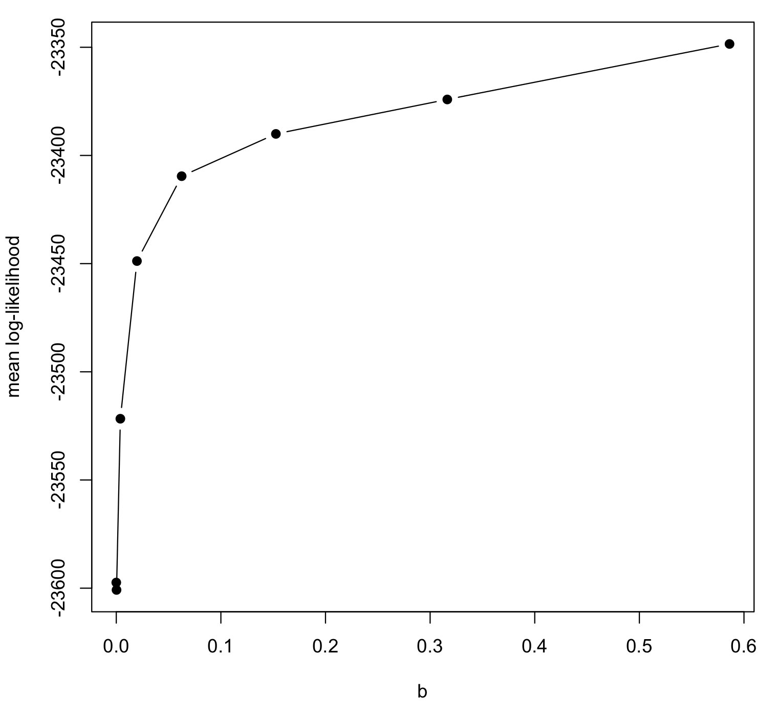
You should obtain a smooth curve increasing from b = 0 towards the right. Any wiggliness in the plot means there may have been convergence problems in the MCMC, or simply that the MCMCs did not run long enough. If you see anything strange with the plot, or if the standard error is too large, you can increase nsample and/or samplefreq to improve the estimates.
The 95% confidence interval of the log-marginal likelihood is
M1$logml + 2 * c(-M1$se, M1$se)
# [1] -23363.13 -23362.46
6. Repeat 2-5 for the M2 model
Create directory ape4s/M2 and copy the bpp.ctl file into it. Edit the file so that the tree looks like
(((gorilla, chimp), human), orang);
That is, we have swapped the positions of gorilla and human so that gorilla is now more closely related to the chimp.
Now repeat steps 3-5:
(3) Select b values. In R:
setwd("../M2") # This assumes you are in ape4s/M1
b = bppr::make.beta(n=8, a=4, method="step-stones")
bppr::make.bfctlf(b, ctlf="bpp.ctl", betaf="beta.txt")
(4) Now run BPP 8 times. In my Mac BASH terminal I do:
# Make sure you are in ape4s/M2
for d in `seq 1 1 8`; do cd $d; bpp -cfile bpp.ctl &>/dev/null & cd ..; done
(5) Collect BPP results and calculate marginal likelihood for M2. In R:
# Make sure R workding directory is now M2
M2 <- bppr::stepping.stones()
M2
# $logml
# [1] -23365.93

# $se
# [1] 0.2044337

# $mean.logl
# [1] -23662.16 -23656.17 -23555.31 -23465.32 -23418.52 -23396.46 -23376.87
# [8] -23348.82

# $b
# [1] 1.000000e-300  2.441406e-04  3.906250e-03  1.977539e-02  6.250000e-02
# [6]  1.525879e-01  3.164062e-01  5.861816e-01
You can see that M1 has a larger marginal likelihood (-23,362.79) than M2 (-23,365.93).
7. Calculate Bayes Factors and posterior model probabilities
We can now convert the marginal likelihoods for M1 and M2 into Bayes factors and the posterior model probabilities. In R:
bppr::bayes.factors(M1, M2)
# $bf
# [1] 1.00000000 0.04335463

# $pr
# [1] 0.95844689 0.04155311
The Bayes factor of M2 over M1 is 0.043 (the first, 1.0, is the Bayes factors of the reference model with itself, i.e. M1 over M1). The relative posterior probability for model M1 is 0.958, while for M2 it is 0.042. These are relative posterior probabilities as we did not test all the possible species-tree models (there are 15 possible rooted trees for 4 species). Thus, we have statistically significant evidence in favour of M1 vs the M2. Because the standard errors for the log-marginal likelihoods are relatively high, your probabilities may show noticeable differences.
If the posterior probabilities for two models are close to 0 or 1, an error of 1 in the log BF may be ok (in other words, we should not care much whether the posterior is 0.999 or 0.9999). If they are moderate, we should like the posterior probabilities to be accurate at the 1% level (that is 0.69 is ok when the correct value is 0.70). In this case the log BF should be accurate at the 0.01 level. Because exp(x) = 1 + x when x is close to 0, the error in log BF becomes the relative error in BF or posterior probabilities (thanks to Ziheng Yang for this note).
[ Update – Feb 2020: Function bayes.factors now performs parametric bootstrap of posterior probabilities, so you should see an element called $pr.ci with the confidence intervals for the posterior probabilities. ]
Exercise: The standard errors for the estimated log-marginal likelihoods are 0.17 and 0.20 for models M1 and M2 respectively. These values are rather high. Modify the bpp.ctl file and increase samplefreq = 40 and nsample = 20000. Run the analysis again and re-calculate the log-marginal likelihoods and standard errors. Roughly, you may want twice the sum of the standard errors to be much smaller than the difference between the log-likelihoods for the two models. How much smaller are the standard errors for the new analysis? Are the calculated posterior probabilities different?
Exercise: In the example above we compared two speciation models. You can test for a third model, M3, in which human and chimp are assummed to be the same species. Create a directory called ape4s/M3 and copy the bpp.ctl file over. Edit the file, and any other input BPP files as appropriate so that BPP considers human and chimp to be two individuals from the same species. You may want to do the tutorial in Yang (2015) if you are not familiar with species delimitation in BPP.
Exercise (harder): bppr also implements thermodynamic integration by Gaussian quadrature (Rannala and Yang, 2017). Repeat the Bayes factors calculations using this technique (check the help files for functions gauss.quad and make.beta in the package).
Bibliography
-
Burgess, R. and Z. Yang. 2008 Estimation of hominoid ancestral population sizes under Bayesian coalescent models incorporating mutation rate variation and sequencing errors. Molecular Biology and Evolution, 25: 1979-1994.
-
Flouri T, Xiyun J, Rannala B, Yang Z. 2018. Species tree inference with BPP using genomic sequences and the multispecies coalescent. Mol Biol Evol.
-
Rannala, B., and Z. Yang. 2017. Efficient Bayesian species tree inference under the multispecies coalescent. Systematic Biology, 66: 823-842.
-
Xie et al. (2011) Improving marginal likelihood estimation for Bayesian phylogenetic model selection. Systematic Biology, 60: 150–160.
-
Yang (2014) Molecular Evolution: A Statistical Approach. Oxford University Press.
-
Yang, Z. 2015. The BPP program for species tree estimation and species delimitation. Current Zoology, 61: 854-865.