Bayes (1763) analyses the following thought experiment: A ball is thrown onto a table, and the position of the ball is marked. A second ball is thrown, repeatedly, on the table. We record, after each throw, whether the second ball fell on the left or right of the first ball. Bayes (1763) worked out the conditional probability of the position of the first ball given the sequence of throws of the second ball. This probability, which we would now call a posterior distribution, is given by the beta distribution.

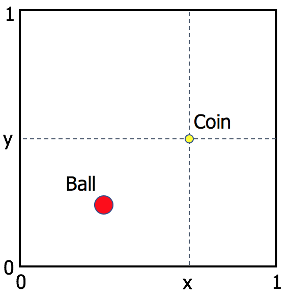
I was invited to give an introduction to Bayesian phylogenetics at the 2019 Phylogenomics Workshop in Cesky Krumlov, and I thought it would be fun to run a simulation of Bayes original thought experiment. I modified the experiment a bit: Assume an even and perfectly smooth 1m × 1m table. The first ball is thrown and a coin is used to mark the position of the ball. The coordinates of the coin are x (the perpendicular distance from the left edge of the table) and y (the perpendicular distance from the front edge of the table). The ball is repeatedly thrown on the table, and we are told whether it fell on the left or right and on the front or back of the coin. We are never allowed to see the ball being thrown or its position on the table. We must guess where the coin is from our record of lefts/rights and fronts/backs after n throws. The figure below shows a diagram of the table and the coin.

We assume the position of the coin has the joint uniform distribution, f(x, y) = 1. Let T_n be the sequence of outcomes after n throws. For example, T₃ = ({L,F}, {L,F}, {R,B}) means the ball landed on the left and front of the coin on the first two throws and on the right and back in the last throw. The posterior distribution of x and y given T_n is the joint beta distribution:

Pr(x, y | T_n) = x^a (1 – x)^{n – a} y^a (1 – y)^{n – y} / Pr(T_n),

where

Pr(T_n) = a! (n – a)! b! (n – b)! / (n – 1)!²

and a, b, are the number of times the ball fell on the left and front of the coin, respectively, and n is the total number of throws.

The R code below can be used to recreate the modified Reverend Bayes ball and table experiment. The first lines of code define the posterior distribution and the normalisation constant, 1 / Pr(T_n). The simulation for n = 30 throws of the ball then takes place. The first for loop plots the contour of the posterior as the number of throws goes from n = 0 to n = 30. The second for loop gives the perspective plots of the posterior as the number of throws goes from n = 0 to n = 30. The posterior surface for n = 30 may look like this (different runs of the code will produce different simulation outcomes):

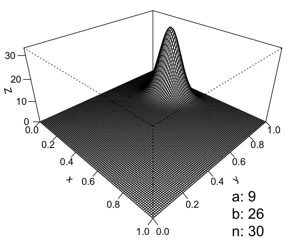
If you run the R code you can see the perspective plot evolving from the prior, f(x,y) = 1, for n = 0, into the bell-shaped posterior for n = 30. This bell-shaped posterior is our best guess about the position of the coin. It turns out to be a very good guess!

# Bayes modified ball and table experiment
# Cesky-Krumlov phylogenomics workshop, Jan 2019
# (c) Mario dos Reis, 2019
# You can reuse this code under the terms of the MIT license
# https://opensource.org/licenses/MIT
rm(list=ls())

# Joint un-normalised posterior of x, y coordinates of first ball (coin)
# P(x,y|Tn) * P(Tn):
# Prior is f(x,y) = 1
# pos: number of times second ball fell left and front of first
# n: number of throws of second ball
# N: number of divisions for density grid (z is NxN)
# Returns matrix z of un-normalised joint of x and y
jointf <- function(pos, n, N=100) {
  a <- pos[1]; b <- pos[2]
  x <- y <- seq(from=0, to=1, len=N)
  xf <- x^a * (1-x)^(n-a)
  yf <- y^b * (1-y)^(n-b)
  z <- xf %o% yf
}

# Function to calculate normalisation constant, 1/P(Tn):
Cf <- function(x, y, n) {
  ( factorial(n+1) )^2 /
  ( factorial(x) * factorial(n-x) * factorial(y) * factorial(n-y) )
}

# Throw first ball, mark with a coin, then second ball n times
n <- 30
xy <- runif(2) # position of coin after intial throw
xy.2 <- matrix(runif(2 * n), ncol=2) # additional n throws of the ball

# positions (is the second ball to the left or front of the coin?):
pos <- numeric(2)
pos[1] <- sum(xy.2[,1] < xy[1])
pos[2] <- sum(xy.2[,2] < xy[2])

# To reproduce lecture slides use:
# xy <- c(0.2789525, 0.8635796)
# pos <- c(9, 26)

# Posterior, f(x,y|Tn):
z <- jointf(pos, n) * Cf(pos[1], pos[2], n)
#persp(z, box=TRUE, tick="det", theta=45, phi=30, expand=.5)
image(-z, las=1); contour(z, add=TRUE)
#dev2bitmap("2d-cesky.1.png", height=6, width=6, res=300, type="png16")
# Position of coin:
abline(v=xy[1], h=xy[2], lty=2)
points(xy[1], xy[2], cex=2, pch=19, col="white"); points(xy[1], xy[2], cex=2)
#dev2bitmap("2d-cesky.2.png", height=6, width=6, res=300, type="png16")
# Positions of each of the n throws:
points(xy.2[,1], xy.2[,2], pch=19)
#dev2bitmap("2d-cesky.3.png", height=6, width=6, res=300, type="png16")

# calculate cumulative positions to make posterior plot animation:
xpos <- cumsum(xy.2[,1] < xy[1])
ypos <- cumsum(xy.2[,2] < xy[2])
# To reproduce lecture slides use:
#xpos <- c(0,0,1,1,1,2,2,3,3,3,4,5,5,5,5,5,5,5,6,6,6,7,7,7,7,7,7,8,8,9)
#ypos <- c(1,2,3,4,5,5,6,7,8,9,10,10,11,12,13,14,15,16,17,18,19,20,20,21,22,23,24,25,25,26)
xypos <- cbind(xpos, ypos)
#save.image("Cesky.RData")

# contour plot after each throw:
z <- jointf(c(0,0), 0)
image(-z); contour(z, nlevels=10, drawlabels=FALSE, add=TRUE)
for (i in 1:n) {
  # If locator() is uncommented, you must click on the image with your mouse
  # to see each plot:
  #locator(1)
  z <- jointf(xypos[i,], i)
  image(z); contour(z, nlevels=10, drawlabels=FALSE, add=TRUE)
}

# perspective plot after each throw (this matches the lectures slides):
zlim=c(0, 33)
z <- jointf(c(0,0), 0)
persp(z, box=TRUE, tick="det", theta=45, phi=30, expand=.5, zlim=zlim, xlab="x", ylab="y")
legend(.18, -.28, paste("a:", 0, "\nb:", 0, "\nn:", 0), bty="n", cex=1.5)
#dev2bitmap("cesky-0.png", res=300, ty="pngmono") # saves plot to a file
for (i in 1:n) {
  # if locator() is uncommented, you must click on the image with your mouse
  # to see the next plot:
  #locator(1)
  C <- Cf(xpos[i], ypos[i], i) # 1/P(Tn)
  z <- jointf(xypos[i,], i) * C # z * C = f(x,y|Tn)
  persp(z, box=TRUE, tick="det", theta=45, phi=30, expand=.5, zlim=zlim, xlab="x", ylab="y")
  legend(.18, -.28, paste("a:", xpos[i], "\nb:", ypos[i], "\nn:", i), bty="n", cex=1.5)
  # saves plot to a file:
  #dev2bitmap(paste("cesky-", i, ".png", sep=""), res=300, ty="pngmono")
}

References

Bayes, T (1763) An essay towards solving a problem in the doctrine of chances. Phil. Transc. R. Soc. 53: 370. DOI: 10.1098/rstl.1763.0053